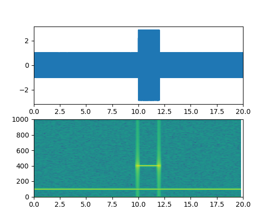
Axes.specgram(x, NFFT=None, Fs=None, Fc=None, detrend=None, window=None, noverlap=None, cmap=None, xextent=None, pad_to=None, sides=None, scale_by_freq=None, mode=None, scale=None, vmin=None, vmax=None, **kwargs)¶Plot a spectrogram.
Call signature:
specgram(x, NFFT=256, Fs=2, Fc=0, detrend=mlab.detrend_none,
         window=mlab.window_hanning, noverlap=128,
         cmap=None, xextent=None, pad_to=None, sides='default',
         scale_by_freq=None, mode='default', scale='default',
         **kwargs)
Compute and plot a spectrogram of data in x. Data are split into NFFT length segments and the spectrum of each section is computed. The windowing function window is applied to each segment, and the amount of overlap of each segment is specified with noverlap. The spectrogram is plotted as a colormap (using imshow).
Keyword arguments:
- Fs: scalar
- The sampling frequency (samples per time unit). It is used to calculate the Fourier frequencies, freqs, in cycles per time unit. The default value is 2.
- window: callable or ndarray
- A function or a vector of length NFFT. To create window vectors see
window_hanning(),window_none(),numpy.blackman(),numpy.hamming(),numpy.bartlett(),scipy.signal(),scipy.signal.get_window(), etc. The default iswindow_hanning(). If a function is passed as the argument, it must take a data segment as an argument and return the windowed version of the segment.- sides: [ ‘default’ | ‘onesided’ | ‘twosided’ ]
- Specifies which sides of the spectrum to return. Default gives the default behavior, which returns one-sided for real data and both for complex data. ‘onesided’ forces the return of a one-sided spectrum, while ‘twosided’ forces two-sided.
callable
The function applied to each segment before fft-ing,
designed to remove the mean or linear trend. Unlike in
MATLAB, where the detrend parameter is a vector, in
matplotlib is it a function. The pylab
module defines detrend_none(),
detrend_mean(), and
detrend_linear(), but you can use
a custom function as well. You can also use a string to choose
one of the functions. ‘default’, ‘constant’, and ‘mean’ call
detrend_mean(). ‘linear’ calls
detrend_linear(). ‘none’ calls
detrend_none().
Specifies whether the resulting density values should be scaled by the scaling frequency, which gives density in units of Hz^-1. This allows for integration over the returned frequency values. The default is True for MATLAB compatibility.
matplotlib.colors.Colormap instance; if None, use
default determined by rcspecgram()Note
detrend and scale_by_freq only apply when mode is set to ‘psd’
Returns the tuple (spectrum, freqs, t, im):
- spectrum: 2-D array
- columns are the periodograms of successive segments
- freqs: 1-D array
- The frequencies corresponding to the rows in spectrum
- t: 1-D array
- The times corresponding to midpoints of segments (i.e the columns in spectrum)
- im: instance of class
AxesImage- The image created by imshow containing the spectrogram
Example:
(Source code, png, pdf)

See also
psd()psd() differs in the default overlap; in returning
the mean of the segment periodograms; in not returning
times; and in generating a line plot instead of colormap.magnitude_spectrum()angle_spectrum()phase_spectrum()Notes
In addition to the above described arguments, this function can take a data keyword argument. If such a data argument is given, the following arguments are replaced by data[<arg>]: